Downstream Analysis: CRG Identification, Alteration Type Disentanglement & CRR Delineation
This notebook performs three downstream analyses after SILPAG model training:
Task 1: CRG Identification — Identify condition-responsive genes.
Task 2: Alteration Type Disentanglement — Determine the nature of each CRG’s alteration.
Task 3: CRR Delineation — Delineate condition-responsive tissue regions.
Prerequisites: A trained SILPAG model saved from Getting Started with SILPAG.
0. Setup
[1]:
import warnings
warnings.filterwarnings('ignore')

import scanpy as sc
import anndata as ad
import numpy as np
import pandas as pd
import torch
from scipy import sparse
import matplotlib.pyplot as plt
import seaborn as sns
import matplotlib

import SILPAG as sp
1. Load Data & Preprocessing
Same preprocessing as Getting Started with SILPAG — load reference (normal breast) and target (breast cancer), intersect genes, filter.
[2]:
ref = sc.read_h5ad('SILPAG/data/V02_nb.h5ad')
adata = sc.read_h5ad('SILPAG/data/H1_nb.h5ad')
ref.var_names_make_unique()
adata.var_names_make_unique()
sp.prefilter_specialgenes(ref)
sp.prefilter_specialgenes(adata)

gene = list(set(ref.var_names) & set(adata.var_names))
ref = ref[:, gene]
adata = adata[:, gene]

g1 = sc.pp.filter_genes(ref, min_cells=int(ref.shape[0] * 0.02), inplace=False)
g2 = sc.pp.filter_genes(adata, min_cells=int(adata.shape[0] * 0.02), inplace=False)
ref = ref[:, g1[0] | g2[0]]
adata = adata[:, g1[0] | g2[0]]

key = list(set(ref.var_names) & set(adata.var_names))
ref = ref[:, key]
adata = adata[:, key]
ref.var['hkgene'] = adata.var['hkgene']

labels = np.zeros(ref.shape[1], dtype=int)
labels[np.where(ref.var['hkgene'] == 1)[0]] = 1
del ref.raw

print(f'Reference: {ref.shape}, Target: {adata.shape}')
Reference: (1896, 7874), Target: (613, 7874)
2. Load Trained Model & Generate View-Transferred SGMs
Load the saved model, compute the codebook transport plan, and generate:
result1: view-transferred SGM (reference \(\rightarrow\) target via OT)result2: target self-reconstruction
[3]:
# Load saved config first so that patch_size, K, img_size etc. are restored
args = sp.Config.load_config('SILPAG/saved_model/hBC_demo')
args.device = 'cuda:7'
args.train = False

# Clear size lists — GeneDataset will re-populate them from the actual data
args.orig_img_size = []
args.resized_img_size = []
args.img_size = []

gene_images = [ref.varm['gene_img'], adata.varm['gene_img']]
train_dataset = sp.GeneDataset(gene_images, labels, args)

from torch.utils.data import DataLoader
train_loader = DataLoader(train_dataset, batch_size=args.batch_size, shuffle=False, drop_last=False)
model, dataset, PI, Q = sp.train_marker(train_loader, hist_data=None, args=args)

print(f'Model loaded. Codebook sizes: {[model.get_codebook(i).shape[0] for i in range(args.num_slice)]}')
Shape of each View:  [(66, 96), (30, 30)]
Model loaded. Codebook sizes: [51, 203]
[4]:
# Compute gene codes via OT transport plan
code = sp.get_code(model, dataset, hist_data=None, pi_init=PI, source_idx=0, target_idx=1, args=args)
adata.varm['code_ref'] = code[0]  # reference -> target (transported)
adata.varm['code_tgt'] = code[1]  # target native

# Generate SGMs
result1 = model.generate(args, adata, tgt_index=1, code_id='code_ref', gene='all')  # view-transferred
result2 = model.generate(args, adata, tgt_index=1, code_id='code_tgt', gene='all')  # target self-recon

print(f'Generated SGMs: {result1.shape}, {result2.shape}')
Generating...: 100%|██████████| 7874/7874 [00:07<00:00, 1017.53gene/s]
Generating...: 100%|██████████| 7874/7874 [00:07<00:00, 992.01gene/s]
Generated SGMs: (613, 7874), (613, 7874)
Task 1: CRG Identification
For each gene \(i\), compute the CRG score:
The anchor gene scores form an empirical null modelled as \(S \sim \Gamma(k, \theta)\). Genes with \(p < 0.05\) are designated as CRGs.
[5]:
# Compute CRG scores
scores = sp.compute_crg_scores(result1, adata)

# Anchor mask from training
anchor_mask = dataset.labels.astype(bool)
print(f'Total genes: {len(scores)}, Anchor genes: {anchor_mask.sum()}')

# Identify CRGs
# null_model='gamma': fits Gamma distribution to anchor scores
# No FDR correction — use raw p-value directly
crg_result = sp.identify_crgs(
    scores, anchor_mask,
    p_threshold=0.1,
    null_model='gamma',
    correction=None,
)

n_crg = crg_result['is_crg'].sum()
print(f'Identified {n_crg} CRGs (p < 0.05, null_model=gamma, no FDR)')
print(f'Null info: {crg_result["null_info"]}')
Total genes: 7874, Anchor genes: 1914
Identified 193 CRGs (p < 0.05, null_model=gamma, no FDR)
Null info: {'model': 'gamma', 'k': 0.4509458695722796, 'loc': 0, 'theta': np.float32(2338.6943)}
Store CRG Results in AnnData
[6]:
adata.var['crg_score'] = scores
adata.var['crg_pval'] = crg_result['pvalues']
adata.var['crg_fdr'] = crg_result['pvalues_adj']
adata.var['is_crg'] = crg_result['is_crg']

crg_genes = adata.var_names[crg_result['is_crg']]
print(f'Top 20 CRGs by score:')
adata.var.loc[crg_genes].sort_values('crg_score', ascending=False).head(20)[['crg_score', 'crg_fdr']]
Top 20 CRGs by score:
[6]:
| crg_score | crg_fdr | |
|---|---|---|
| IGKC | 6.109030e+06 | 0.000000e+00 |
| IGHA1 | 3.070430e+06 | 0.000000e+00 |
| IGHG4 | 1.892223e+06 | 0.000000e+00 |
| IGHG3 | 7.547800e+05 | 0.000000e+00 |
| IGLC3 | 4.252860e+05 | 0.000000e+00 |
| TMSB10 | 3.985322e+05 | 0.000000e+00 |
| IGLC2 | 1.883705e+05 | 0.000000e+00 |
| RACK1 | 1.202756e+05 | 0.000000e+00 |
| ERBB2 | 1.130827e+05 | 0.000000e+00 |
| GAPDH | 1.039025e+05 | 0.000000e+00 |
| MGP | 1.028431e+05 | 0.000000e+00 |
| IGHG1 | 9.073847e+04 | 0.000000e+00 |
| S100A9 | 8.803026e+04 | 0.000000e+00 |
| PFN1 | 5.699932e+04 | 2.245537e-12 |
| ACTB | 5.231029e+04 | 1.744782e-11 |
| UBA52 | 4.986116e+04 | 5.099254e-11 |
| SSR4 | 3.802821e+04 | 9.255538e-09 |
| CD74 | 3.611092e+04 | 2.158245e-08 |
| KRT19 | 3.067662e+04 | 2.397699e-07 |
| CST3 | 2.966526e+04 | 3.759009e-07 |
Task 2: Alteration Type Disentanglement
For each CRG, three statistical tests determine the nature of the alteration:
Test |
What it detects |
Method |
|---|---|---|
Differential Abundance |
Shift in expression magnitude |
Wilcoxon rank-sum |
Differential Prevalence |
Change in fraction of expressing spots |
Fisher’s exact (binarised at \(\epsilon\)) |
Differential Spatial Pattern |
Structured spatial discrepancy |
Moran’s I permutation on SDM |
A gene can be assigned to multiple alteration types.
[7]:
df_alt = sp.disentangle_alteration_types(
    result_ref=result1,
    adata=adata,
    crg_mask=crg_result['is_crg'],
    epsilon=0.01,              # binarisation threshold for prevalence
    n_neighbors=15,
    fdr_threshold=0.05,
    abundance_effect_size=1,
    spatial_I_threshold=0.5,   # require Moran's I >= 0.1 for spatial
)

print(f'Disentanglement results for {len(df_alt)} CRGs:')
print(df_alt[['is_diff_abundance', 'is_diff_prevalence', 'is_diff_spatial']].sum())
Disentanglement results for 193 CRGs:
is_diff_abundance     95
is_diff_prevalence    47
is_diff_spatial       62
dtype: int64
Detailed Results Table
[8]:
# Merge CRG scores into the disentanglement table
df_alt['crg_score'] = adata.var.loc[df_alt.index, 'crg_score'].values
df_alt['crg_fdr'] = adata.var.loc[df_alt.index, 'crg_fdr'].values

df_display = df_alt.sort_values('crg_score', ascending=False)
df_display[['crg_score', 'crg_fdr', 'abundance_fdr', 'prevalence_fdr', 'spatial_fdr']].head(15)
[8]:
| crg_score | crg_fdr | abundance_fdr | prevalence_fdr | spatial_fdr | |
|---|---|---|---|---|---|
| gene | |||||
| IGKC | 6.109030e+06 | 0.000000e+00 | 0.000000e+00 | 1.0 | 0.0 |
| IGHA1 | 3.070430e+06 | 0.000000e+00 | 0.000000e+00 | 1.0 | 0.0 |
| IGHG4 | 1.892223e+06 | 0.000000e+00 | 0.000000e+00 | 1.0 | 0.0 |
| IGHG3 | 7.547800e+05 | 0.000000e+00 | 0.000000e+00 | 1.0 | 0.0 |
| IGLC3 | 4.252860e+05 | 0.000000e+00 | 0.000000e+00 | 1.0 | 0.0 |
| TMSB10 | 3.985322e+05 | 0.000000e+00 | 0.000000e+00 | 1.0 | 0.0 |
| IGLC2 | 1.883705e+05 | 0.000000e+00 | 0.000000e+00 | 1.0 | 0.0 |
| RACK1 | 1.202756e+05 | 0.000000e+00 | 0.000000e+00 | 1.0 | 0.0 |
| ERBB2 | 1.130827e+05 | 0.000000e+00 | 7.353808e-286 | 1.0 | 0.0 |
| GAPDH | 1.039025e+05 | 0.000000e+00 | 0.000000e+00 | 1.0 | 0.0 |
| MGP | 1.028431e+05 | 0.000000e+00 | 3.347538e-280 | 1.0 | 0.0 |
| IGHG1 | 9.073847e+04 | 0.000000e+00 | 0.000000e+00 | 1.0 | 0.0 |
| S100A9 | 8.803026e+04 | 0.000000e+00 | 0.000000e+00 | 1.0 | 0.0 |
| PFN1 | 5.699932e+04 | 2.245537e-12 | 1.087336e-297 | 1.0 | 0.0 |
| ACTB | 5.231029e+04 | 1.744782e-11 | 2.150568e-265 | 1.0 | 0.0 |
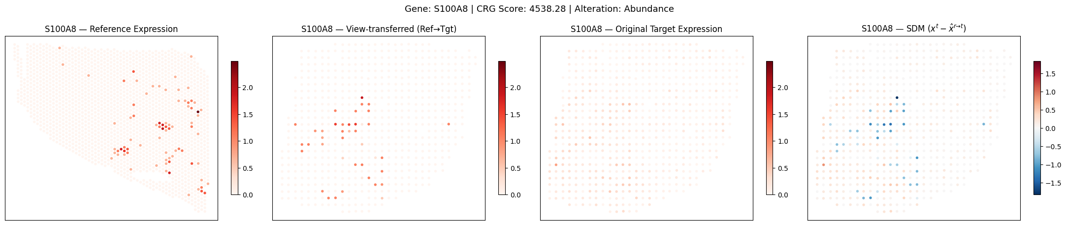
Example CRG Visualisation
Visualise the reference expression, view-transferred SGM, target self-reconstruction, and SDM.
[9]:
# Visualise
top_gene = 'S100A8'
gene_idx = list(adata.var_names).index(top_gene)

X_ref_sgm = result1.X.toarray() if sparse.issparse(result1.X) else np.array(result1.X)

# Reference slice: original expression on reference coordinates
ref_expr = ref.X.toarray()[:, gene_idx] if sparse.issparse(ref.X) else np.array(ref.X)[:, gene_idx]
ref_coords = ref.obsm['spatial']

# Target slice
tgt_coords = adata.obsm['spatial']
expr_vt = X_ref_sgm[:, gene_idx]      # view-transferred

# Original target expression
tgt_raw = adata.X.toarray()[:, gene_idx] if sparse.issparse(adata.X) else np.array(adata.X)[:, gene_idx]

# Normalize (library-size) + log1p before visualisation
def _norm_log(x):
    total = x.sum()
    if total > 0:
        x = x / total * np.median([ref_expr.sum(), expr_vt.sum(), tgt_raw.sum()])
    return np.log1p(x)

ref_expr = _norm_log(ref_expr)
expr_vt  = _norm_log(expr_vt)
tgt_raw  = _norm_log(tgt_raw)

sdm = tgt_raw - expr_vt               # SDM: original target - view-transferred

fig, axes = plt.subplots(1, 4, figsize=(22, 4.5))

# Unified color scale for expression panels
vmin_expr = 0
vmax_expr = max(ref_expr.max(), expr_vt.max(), tgt_raw.max())

# Panel 0: Reference expression (on reference coordinates)
sc0 = axes[0].scatter(ref_coords[:, 0], ref_coords[:, 1], c=ref_expr, s=8, cmap='Reds', vmin=vmin_expr, vmax=vmax_expr)
axes[0].set_title(f'{top_gene} — Reference Expression')
axes[0].set_aspect('equal')
axes[0].invert_yaxis()
plt.colorbar(sc0, ax=axes[0], shrink=0.7)

# Panel 1: View-transferred SGM (on target coordinates)
sc1 = axes[1].scatter(tgt_coords[:, 0], tgt_coords[:, 1], c=expr_vt, s=8, cmap='Reds', vmin=vmin_expr, vmax=vmax_expr)
axes[1].set_title(f'{top_gene} — View-transferred (Ref→Tgt)')
axes[1].set_aspect('equal')
axes[1].invert_yaxis()
plt.colorbar(sc1, ax=axes[1], shrink=0.7)

# Panel 2: Original target expression (on target coordinates)
sc2 = axes[2].scatter(tgt_coords[:, 0], tgt_coords[:, 1], c=tgt_raw, s=8, cmap='Reds', vmin=vmin_expr, vmax=vmax_expr)
axes[2].set_title(f'{top_gene} — Original Target Expression')
axes[2].set_aspect('equal')
axes[2].invert_yaxis()
plt.colorbar(sc2, ax=axes[2], shrink=0.7)

# Panel 3: SDM (symmetric scale)
vlim = max(abs(sdm.min()), abs(sdm.max()))
sc3 = axes[3].scatter(tgt_coords[:, 0], tgt_coords[:, 1], c=sdm, s=8, cmap='RdBu_r', vmin=-vlim, vmax=vlim)
axes[3].set_title(f'{top_gene} — SDM ($x^t - \\hat{{x}}^{{r→t}}$)')
axes[3].set_aspect('equal')
axes[3].invert_yaxis()
plt.colorbar(sc3, ax=axes[3], shrink=0.7)

for ax in axes:
    ax.set_xticks([])
    ax.set_yticks([])

if top_gene in df_alt.index:
    alt_type = df_alt.loc[top_gene, 'alteration_type']
else:
    alt_type = 'N/A'
fig.suptitle(f'Gene: {top_gene} | CRG Score: {scores[gene_idx]:.2f} | Alteration: {alt_type}', fontsize=13, y=1.02)
plt.tight_layout()
plt.show()
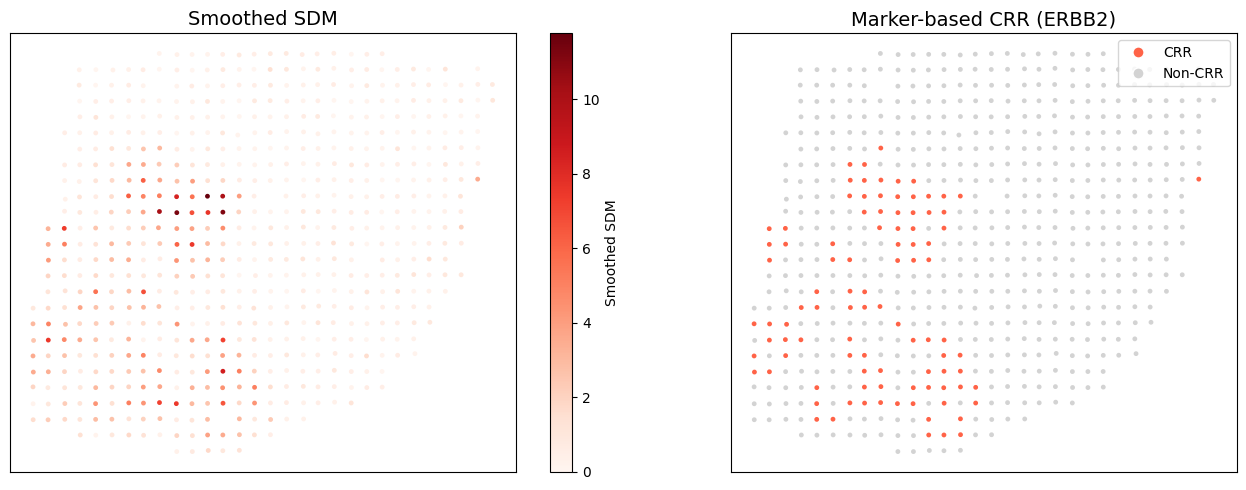
Task 3: CRR Delineation
Delineate condition-responsive tissue regions (CRR) using two approaches:
Marker-based: For a known condition-associated gene \(g\), compute the SDM \(D_g = |\hat{\mathbf{x}}^{r \to t}_g - \mathbf{x}^t_g|\), smooth with a Gaussian kernel (\(\sigma=1\)), then apply Otsu’s method to find the optimal threshold \(\tau^*\) that maximises between-group variance.
Marker-free: When no markers are available, use all CRGs. Each spot \(i\) gets a discrepancy vector \(\mathbf{f}_i \in \mathbb{R}^{|I_{CRG}|}\). Leiden clustering on \(\{\mathbf{f}_i\}\) yields two spatial domains; the CRR is the one with higher aggregate discrepancy.
Marker-based CRR Delineation
Use ERBB2 as the marker gene to delineate the CRR.
[10]:
# Marker-based delineation with ERBB2
marker_gene = 'ERBB2'
print(f'Marker gene for CRR delineation: {marker_gene}')

crr_marker = sp.delineate_crr_marker(
    result_ref=result1,
    adata=adata,
    gene=marker_gene,
    sigma=1.0,
)

n_crr = crr_marker['crr_mask'].sum()
print(f'CRR spots: {n_crr}/{len(crr_marker["crr_mask"])} '
      f'(Otsu threshold: {crr_marker["threshold"]:.2f})')

# Visualise
sp.plot_crr(
    coords=crr_marker['coords'],
    crr_mask=crr_marker['crr_mask'],
    sdm_smoothed=crr_marker['sdm_smoothed'],
    title=f'Marker-based CRR ({marker_gene})',
)
Marker gene for CRR delineation: ERBB2
CRR spots: 96/613 (Otsu threshold: 2.70)
Store CRR Results
[11]:
# Store CRR annotations in adata.obs
adata.obs['crr_marker'] = crr_marker['crr_mask'].astype(int)
adata.obs['crr_marker_sdm'] = crr_marker['sdm_smoothed']

print(f'Marker-based CRR: {adata.obs["crr_marker"].sum()} spots')
Marker-based CRR: 96 spots
Save All Results
[12]:
# Save disentanglement table
df_alt.to_csv('crg_disentanglement_results.csv')

# Save full gene-level results
adata.var[['crg_score', 'crg_pval', 'crg_fdr', 'is_crg']].to_csv('crg_identification_results.csv')

# Save GO enrichment results
# df_pathway.to_csv('crg_pathway_enrichment_results.csv', index=False)

# Save CRR results
adata.obs[['crr_marker', 'crr_marker_sdm']].to_csv('crr_delineation_results.csv')

print('All results saved.')
All results saved.